Matthew Weinschenk
MNIST Handwritten Digits with KNN and Random Forest in R
The document explores several ways to use R to classify handwritten digits using the classic MNIST handwritten digit data set.
For more information on the data and ML approaches, you should check out the original source which includes a summary of different ML techniques and the resulting accuracy.
The Data
The MNIST data is a collection of 42,000 samples of handwritten digits labeled for the proper output value. The data is already split into a training set and test set.
I’ll download the data from Kaggle as it already contains some helpful preprocessing. Each entry contains the value that’s being written in the first column. The remaining 784 columns represent the grayscale values for pixels for the representation of a 28 x 28 matrix. We’ll choose a random subset of the data to explore more efficiently, and then display part of the first line.
We’re going to use just a small subset of that data, 1,000 observations, so we don’t have to wait so long for processing.
The data comes with a training and a blind test set, so we’ll need to create our own test set as well. Using the caret package makes it quick (more on caret later).
library(caret)
data <- read.csv("train.csv")
data$label <- as.factor(data$label)
set.seed(15)
data.sample <- data[sample(1:nrow(data), 1000, replace=FALSE),]
trainIndex <- createDataPartition(data.sample$label, p=.8, list=FALSE, times=1)
train <- data.sample[trainIndex,]
test <- data.sample[-trainIndex,]

train[1, 1]
## [1] 3
## Levels: 0 1 2 3 4 5 6 7 8 9train[1,340:346]## pixel338 pixel339 pixel340 pixel341 pixel342 pixel343 pixel344
## 25289 0 146 30 0 0 0 0We can see the first entry is a drawing of the number 3 by the label. Some of the pixels in that range have values that indicate dark spots, but many are zero.
What does the “3” look like? We can plot it:
plot_1 <- as.matrix(train[1, 2:785])
dim(plot_1) = c(28,28)
image(plot_1[ ,nrow(plot_1):1], col=gray(255:0/255))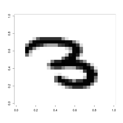
To get a sense of the problem, let’s look at a handful of other 3’s in the dataset.
train.threes <- subset(train, train$label ==3)
par (mfrow =c(4,4), mai=c(0,0,0,0))
for (i in 1:16){
  x = as.matrix(train.threes[i, 2:785])
  dim(x) = c(28,28)
  image(x[,nrow(x):1], col=gray(255:0/255))
  }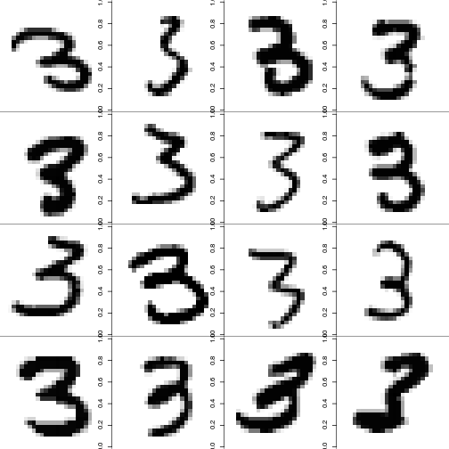
They look pretty different. However, we can see what we’re looking for by plotting the average of each digit.
par(mfrow = c(4,3), mai=c(0,0,0,0))
image_matrix <- array(dim=c(10,28*28))
for (digit in 0:9){
  image_matrix[digit + 1,] <- apply(train[train[,1]==digit, -1], 2, sum)
  image_matrix[digit + 1,] <- image_matrix[digit + 1, ] / max(image_matrix[digit + 1,])*255


  ximg <- as.matrix(image_matrix[digit + 1,])
  dim(ximg) <- c(28,28)
  image(ximg[,nrow(ximg):1], col=gray(255:0/255))
}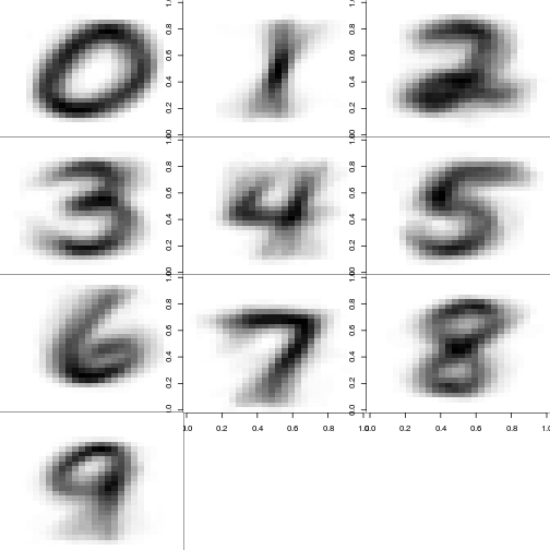
Remember, we’re just using a sample. Were we to use all 42k points, these would get a bit clearer.
Let’s us a K-nearest neighbor algorithm to read new new values.
K-Nearest Neighbors
As the garden-variety classification algorithm, let’s start with KNN. We’ll use the caret package. We’re going to use our small sample and simplify our sampling techniques and parameter ranges so we don’t have to wait forever for computing. If we were looking deeper and had the time we’d be a little more focused on our cross-validation and k choices.
You can think of the caret package like a mega-package of ML algorithms (currently 230). It makes preprocessing and partitioning easy and sets a workflow so you can try different algos on the same dataset without starting from scratch. It even tests various values of ‘k’ for best fit.
To improve our compute time, we’ll use our multicore processor doMC package only works on Linux and make sure you set the number of cores right. If you have questions, just skip this.
library(doMC)
registerDoMC(cores = 4)
We’re going to use cross-validation with 10 folds. On each, we’ll try setting k to all the values from 1 to 10 (by steps of 1).
library(caret)
ctrl <- trainControl(method="cv", number=10)
knn_grid <- expand.grid(k=seq(1,10,1))
knn_fit <- train(label ~., data=train, method="knn", trControl = ctrl, tuneGrid=knn_grid)
The resulting model suggest that k=6 is the best parameter. It’s got an accuracy of 86%. Which isn’t too bad. We can also see from the plot that accuracy increases as k goes from 2 to 6 and then starts to decline.
knn_fit## k-Nearest Neighbors
##
## 805 samples
## 784 predictors
## 10 classes: '0', '1', '2', '3', '4', '5', '6', '7', '8', '9'
##
## No pre-processing
## Resampling: Cross-Validated (10 fold)
## Summary of sample sizes: 723, 726, 725, 724, 723, 723, ...
## Resampling results across tuning parameters:
##
## k Accuracy Kappa Accuracy SD Kappa SD
## 1 0.8670264 0.8520261 0.02125981 0.02362810
## 2 0.8282551 0.8088273 0.03727447 0.04151519
## 3 0.8533509 0.8366718 0.02998666 0.03343270
## 4 0.8546178 0.8380779 0.02498329 0.02776106
## 5 0.8556973 0.8392610 0.03160337 0.03517373
## 6 0.8483184 0.8310402 0.03594120 0.04007705
## 7 0.8507108 0.8337277 0.02941045 0.03279060
## 8 0.8444446 0.8267363 0.03705521 0.04130578
## 9 0.8407710 0.8226380 0.03097175 0.03453931
## 10 0.8347050 0.8158835 0.02601026 0.02898868
##
## Accuracy was used to select the optimal model using the largest value.
## The final value used for the model was k = 1.plot(knn_fit)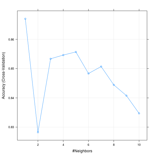
Now we can use the model to predict values of the data we haven’t seen and create a confusion matrix to see how our predicted values match with the actual values.
test$pred <- predict(knn_fit, newdata=test, type="raw")
library(e1071)
confusionMatrix(test$pred, test$label)
## Confusion Matrix and Statistics
##
## Reference
## Prediction 0 1 2 3 4 5 6 7 8 9
## 0 17 0 0 0 0 1 0 0 0 0
## 1 0 21 1 0 1 0 0 1 0 0
## 2 0 2 19 1 0 0 0 0 0 0
## 3 0 0 0 14 0 1 0 0 0 0
## 4 0 0 0 0 14 0 0 0 0 1
## 5 0 0 0 0 0 16 0 0 0 0
## 6 1 0 0 0 0 0 21 0 0 0
## 7 0 0 0 0 0 0 0 16 2 1
## 8 0 0 0 1 0 1 0 0 19 0
## 9 0 0 0 0 1 0 0 3 0 19
##
## Overall Statistics
##
## Accuracy : 0.9026
## 95% CI : (0.852, 0.9403)
## No Information Rate : 0.1179
## P-Value [Acc > NIR] : < 2.2e-16
##
## Kappa : 0.8915
## Mcnemar's Test P-Value : NA
##
## Statistics by Class:
##
## Class: 0 Class: 1 Class: 2 Class: 3 Class: 4 Class: 5
## Sensitivity 0.94444 0.9130 0.95000 0.87500 0.87500 0.84211
## Specificity 0.99435 0.9826 0.98286 0.99441 0.99441 1.00000
## Pos Pred Value 0.94444 0.8750 0.86364 0.93333 0.93333 1.00000
## Neg Pred Value 0.99435 0.9883 0.99422 0.98889 0.98889 0.98324
## Prevalence 0.09231 0.1179 0.10256 0.08205 0.08205 0.09744
## Detection Rate 0.08718 0.1077 0.09744 0.07179 0.07179 0.08205
## Detection Prevalence 0.09231 0.1231 0.11282 0.07692 0.07692 0.08205
## Balanced Accuracy 0.96940 0.9478 0.96643 0.93471 0.93471 0.92105
## Class: 6 Class: 7 Class: 8 Class: 9
## Sensitivity 1.0000 0.80000 0.90476 0.90476
## Specificity 0.9943 0.98286 0.98851 0.97701
## Pos Pred Value 0.9545 0.84211 0.90476 0.82609
## Neg Pred Value 1.0000 0.97727 0.98851 0.98837
## Prevalence 0.1077 0.10256 0.10769 0.10769
## Detection Rate 0.1077 0.08205 0.09744 0.09744
## Detection Prevalence 0.1128 0.09744 0.10769 0.11795
## Balanced Accuracy 0.9971 0.89143 0.94663 0.94089We’ve got a lot of good predictions here. Our overall accuracy is 86.6%. We’ve maybe got a problem telling 1’s from 2’s and 4’s from 9’s, which all make sense given the way those numbers look.
A key tenet of data analysis would not be to use this test data to train our model. That leaves to overfitting. For now, let’s insert the code for if you’d like to train on the entire training set of 30,000 observations. Don’t run this code unless you’re willing to sit and wait for a while. We’ve set eval=FALSE so this code will not run. We’ll also include a timer to see how long it takes.)
timestart <- proc.time()

fullTrainIndex <- createDataPartition(data$label, p=.8, list=FALSE, times=1)
fullTrain <- data[fullTrainIndex,]
fullTest <- data[-fullTrainIndex,]

knn_Fullfit <- train(label ~., data=fullTrain, method="knn", trControl = ctrl, tuneGrid=knn_grid)

timeend <- proc.time()
elapsed <- (timeend - timestart)/60

Print ("Minutes to process:" + elapsed)
And the results:
knn_Fullfit
plot(knn_Fullfit)
Random Forest
With handwriting recognition, we can do better with random forest. Random forest creates a random assortment of decision trees and optimizes which works best. It’s very powerful for classification problems.
With random forest, we’ve got to select the number features to sample at each split (mtry). We’ll try mtry values from 20 to 80 in steps of 10 for our small training set.
library(randomForest)

rf_grid <- expand.grid(mtry= seq(20, 80, 10))
rf_trainControl <- trainControl(method="cv", number = 10)
rf_fit <- train(label ~., data=train, method="rf", trControl=rf_trainControl, tuneGrid = rf_grid)
And look at the results…
rf_fit## Random Forest
##
## 805 samples
## 784 predictors
## 10 classes: '0', '1', '2', '3', '4', '5', '6', '7', '8', '9'
##
## No pre-processing
## Resampling: Cross-Validated (10 fold)
## Summary of sample sizes: 725, 724, 725, 722, 726, 725, ...
## Resampling results across tuning parameters:
##
## mtry Accuracy Kappa Accuracy SD Kappa SD
## 20 0.8992043 0.8878206 0.03536544 0.03933625
## 30 0.8992796 0.8879015 0.03325827 0.03694822
## 40 0.9055311 0.8948517 0.02587492 0.02877404
## 50 0.9004701 0.8892266 0.04057718 0.04512525
## 60 0.9017965 0.8907038 0.04265518 0.04742434
## 70 0.9054392 0.8947531 0.03895305 0.04330188
## 80 0.8916737 0.8794374 0.03983718 0.04428760
##
## Accuracy was used to select the optimal model using the largest value.
## The final value used for the model was mtry = 40.plot(rf_fit)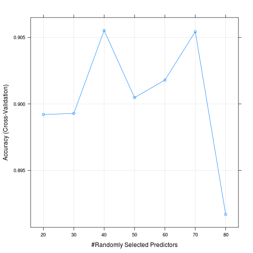
test$pred <- predict(rf_fit, newdata=test, type="raw")
confusionMatrix(test$pred, test$label)
## Confusion Matrix and Statistics
##
## Reference
## Prediction 0 1 2 3 4 5 6 7 8 9
## 0 18 0 0 0 0 1 0 0 0 0
## 1 0 20 2 0 0 0 0 1 0 0
## 2 0 2 17 0 0 0 0 0 0 0
## 3 0 0 0 15 0 0 0 0 0 0
## 4 0 0 0 0 13 0 0 0 0 2
## 5 0 1 1 0 0 17 0 0 1 1
## 6 0 0 0 0 0 0 21 0 0 0
## 7 0 0 0 0 0 1 0 17 0 0
## 8 0 0 0 0 0 0 0 0 20 0
## 9 0 0 0 1 3 0 0 2 0 18
##
## Overall Statistics
##
## Accuracy : 0.9026
## 95% CI : (0.852, 0.9403)
## No Information Rate : 0.1179
## P-Value [Acc > NIR] : < 2.2e-16
##
## Kappa : 0.8916
## Mcnemar's Test P-Value : NA
##
## Statistics by Class:
##
## Class: 0 Class: 1 Class: 2 Class: 3 Class: 4 Class: 5
## Sensitivity 1.00000 0.8696 0.85000 0.93750 0.81250 0.89474
## Specificity 0.99435 0.9826 0.98857 1.00000 0.98883 0.97727
## Pos Pred Value 0.94737 0.8696 0.89474 1.00000 0.86667 0.80952
## Neg Pred Value 1.00000 0.9826 0.98295 0.99444 0.98333 0.98851
## Prevalence 0.09231 0.1179 0.10256 0.08205 0.08205 0.09744
## Detection Rate 0.09231 0.1026 0.08718 0.07692 0.06667 0.08718
## Detection Prevalence 0.09744 0.1179 0.09744 0.07692 0.07692 0.10769
## Balanced Accuracy 0.99718 0.9261 0.91929 0.96875 0.90066 0.93600
## Class: 6 Class: 7 Class: 8 Class: 9
## Sensitivity 1.0000 0.85000 0.9524 0.85714
## Specificity 1.0000 0.99429 1.0000 0.96552
## Pos Pred Value 1.0000 0.94444 1.0000 0.75000
## Neg Pred Value 1.0000 0.98305 0.9943 0.98246
## Prevalence 0.1077 0.10256 0.1077 0.10769
## Detection Rate 0.1077 0.08718 0.1026 0.09231
## Detection Prevalence 0.1077 0.09231 0.1026 0.12308
## Balanced Accuracy 1.0000 0.92214 0.9762 0.91133Caret shows that the best value of mtry that we tried was 20. It’s got an accuracy of nearly 90% on the test data. (And another reminder, this is on a small sample of the data.)
Let’s increase our sample significantly just to show that more data will make the training better. This code may take a while to run, but it’s bearable.
# Take 10,000 observations and partition it.
data.large.sample <- data[sample(1:nrow(data), 10000, replace=FALSE),]
trainIndex2 <- createDataPartition(data.large.sample$label, p=.8, list=FALSE, times=1)
trainLarge <- data.large.sample[trainIndex2,]
testLarge <- data.large.sample[-trainIndex2,]
And train the model
rf_grid_large <- expand.grid(mtry= 20)
rf_largefit <- train(label ~., data=trainLarge, method="rf", trControl=rf_trainControl, tuneGrid = rf_grid_large)
And view the output
rf_largefit## Random Forest
##
## 8004 samples
## 784 predictors
## 10 classes: '0', '1', '2', '3', '4', '5', '6', '7', '8', '9'
##
## No pre-processing
## Resampling: Cross-Validated (10 fold)
## Summary of sample sizes: 7204, 7202, 7204, 7205, 7204, 7206, ...
## Resampling results
##
## Accuracy Kappa Accuracy SD Kappa SD
## 0.9467811 0.9408477 0.009061969 0.0100735
##
## Tuning parameter 'mtry' was held constant at a value of 20
## testLarge$pred <- predict(rf_largefit, newdata=testLarge, type="raw")
confusionMatrix(testLarge$pred, testLarge$label)## Confusion Matrix and Statistics
##
## Reference
## Prediction 0 1 2 3 4 5 6 7 8 9
## 0 197 0 2 0 1 1 2 0 0 2
## 1 0 215 0 0 0 0 0 2 1 0
## 2 0 0 192 6 0 0 1 1 1 0
## 3 0 1 1 193 0 3 0 0 4 1
## 4 1 0 0 0 186 1 0 2 2 2
## 5 0 1 0 4 1 167 1 0 2 0
## 6 0 0 0 0 1 2 193 0 1 0
## 7 0 1 1 1 0 1 0 201 0 1
## 8 0 0 0 2 0 1 2 0 194 2
## 9 0 1 0 1 6 0 0 2 0 185
##
## Overall Statistics
##
## Accuracy : 0.9634
## 95% CI : (0.9542, 0.9712)
## No Information Rate : 0.1097
## P-Value [Acc > NIR] : < 2.2e-16
##
## Kappa : 0.9594
## Mcnemar's Test P-Value : NA
##
## Statistics by Class:
##
## Class: 0 Class: 1 Class: 2 Class: 3 Class: 4 Class: 5 Class: 6
## Sensitivity 0.9949 0.9817 0.97959 0.93237 0.95385 0.94886 0.96985
## Specificity 0.9956 0.9983 0.99500 0.99441 0.99556 0.99505 0.99777
## Pos Pred Value 0.9610 0.9862 0.95522 0.95074 0.95876 0.94886 0.97970
## Neg Pred Value 0.9994 0.9978 0.99777 0.99219 0.99501 0.99505 0.99666
## Prevalence 0.0992 0.1097 0.09820 0.10371 0.09770 0.08818 0.09970
## Detection Rate 0.0987 0.1077 0.09619 0.09669 0.09319 0.08367 0.09669
## Detection Prevalence 0.1027 0.1092 0.10070 0.10170 0.09719 0.08818 0.09870
## Balanced Accuracy 0.9953 0.9900 0.98730 0.96339 0.97470 0.97196 0.98381
## Class: 7 Class: 8 Class: 9
## Sensitivity 0.9663 0.94634 0.95855
## Specificity 0.9972 0.99609 0.99445
## Pos Pred Value 0.9757 0.96517 0.94872
## Neg Pred Value 0.9961 0.99387 0.99556
## Prevalence 0.1042 0.10271 0.09669
## Detection Rate 0.1007 0.09719 0.09269
## Detection Prevalence 0.1032 0.10070 0.09770
## Balanced Accuracy 0.9818 0.97122 0.97650Now we’re up to 95% accuracy on predicting handwritten digits with pretty straightforward, off-the-shelf machine learning algorithms. We could squeeze out a few more basis points by training on the 30,000 observation.
According to some of the best results on this data set, we could do even better using neural networks.
R Session Information
sessionInfo()## R version 3.3.1 (2016-06-21)
## Platform: x86_64-pc-linux-gnu (64-bit)
## Running under: Ubuntu 14.04.2 LTS
##
## locale:
## [1] LC_CTYPE=en_US.UTF-8 LC_NUMERIC=C
## [3] LC_TIME=en_US.UTF-8 LC_COLLATE=en_US.UTF-8
## [5] LC_MONETARY=en_US.UTF-8 LC_MESSAGES=en_US.UTF-8
## [7] LC_PAPER=en_US.UTF-8 LC_NAME=C
## [9] LC_ADDRESS=C LC_TELEPHONE=C
## [11] LC_MEASUREMENT=en_US.UTF-8 LC_IDENTIFICATION=C
##
## attached base packages:
## [1] parallel stats graphics grDevices utils datasets methods base
##
## other attached packages:
## [1] doMC_1.3.4 iterators_1.0.8
## [3] knitr_1.12.3 randomForest_4.6-12
## [5] e1071_1.6-7 caret_6.0-64
## [7] ggplot2_1.0.1 lattice_0.20-33
## [9] DEoptim_2.2-3 devtools_1.12.0
## [11] PortfolioAnalytics_1.0.3636 PerformanceAnalytics_1.4.3541
## [13] foreach_1.4.3 xts_0.9-7
## [15] zoo_1.7-13
##
## loaded via a namespace (and not attached):
## [1] Rcpp_0.12.1 compiler_3.3.1 formatR_1.3 highr_0.5.1
## [5] nloptr_1.0.4 plyr_1.8.3 class_7.3-12 tools_3.3.1
## [9] digest_0.6.8 lme4_1.1-11 evaluate_0.8.3 memoise_1.0.0
## [13] nlme_3.1-125 gtable_0.1.2 mgcv_1.8-6 Matrix_1.2-4
## [17] SparseM_1.7 proto_0.3-10 withr_1.0.2 stringr_1.0.0
## [21] MatrixModels_0.4-1 stats4_3.3.1 grid_3.3.1 nnet_7.3-9
## [25] minqa_1.2.4 reshape2_1.4.1 car_2.1-1 magrittr_1.5
## [29] scales_0.3.0 codetools_0.2-11 MASS_7.3-45 splines_3.3.1
## [33] pbkrtest_0.4-6 colorspace_1.2-6 quantreg_5.21 stringi_1.0-1
## [37] munsell_0.4.2