Matthew Weinschenk
The Question of Urban Renewal
What is the effect of urban renewal and slum clearance? Given the different characteristics of cities its difficult to directly determine the city-wide effects of programs designed to improve certain neighborhoods.
To investigate this question, this document creates linear models in R and descibes the use of instrumental variables as a method of teasing out relations ships by way of replicating a study by William J. Collins and Katherine L. Shester.
The data and paper are available here: American Economic Association
And a free working paper version is available here: NBER
A Brief History
After World War II, Title I of the Housing Act of 1949 offered federal subsidies to cities willing to undertake revitalization projects. The funding ran through 1974, by which time a total of $53 billion (in 2009 money) had been parceled out.
Such projects can be controversial. Opponents complain about unfair impacts on poor residents, such as displacement and the destruction of neighborhoods.
There certainly are such consequences. With this data, we can only investigate whether or not these projects have positive economic effects on the city as a whole.
The Instrumental Variable
Simply comparing the outcomes of cities that underwent renewal projects and those that did not would suffer from selection bias. That is, the cities that chose to undertake renewal projects may have had something fundamentally different about them that would change their subsequent economic outcomes.
For instance, cities that undertook projects may have had more proactive local governments or they may have already had stronger economies.
In an attempt to isolate the effects of the projects, we’ll use an instrumental variable (or instrument). The goal of an instrumental variable is to find a feature that related to your treatment (the use of renewal programs) but not related to the error term of your regression (the variation in economic outcomes.)
Instruments are weird to think about and a better understanding will help many people better interpret statistical findings.
In a classic example, economist Michael Waldman wanted to test if watching television contributed to the development of autism. Ideally, you could test the amount of television watched against rates of autism but we don’t have data on the amount of television watched. Instead he used the amount of rain. If it rains more, children will stay inside and watch more television (the instrument is related to the treatment) but rain does not cause autism (the instrument is unrelated to the outcome).
In the urban renewal case, we can look at local laws that prevented renewal projects as an instrument.
In order to claim the federal funds, states had to enable legislation and create local public agencies (LPAs) to start the renewal programs. If there were legislative delays, a city that wanted to participate would be constrained from participating. When you consider the start date of an LPA, you’re really measuring years of potential participation in renewal programs.
We’re trying to remove the effect of cities self-selecting for renewal projects. So cities being contrained by laws (the instrument) is related to the undertaking of renewal projects (the treatment) but unrelated to the other economic starting conditions of the city (the variation in the outcome).
The Data
The data includes cities with more than 25,000 residents, lists the total of federal grants by the end of the program in 1974, and includes a range of different housing and economic data at 1950 and 1980.
## The data comes in the dta file format for Stata. To read in R...
library(foreign)
data <- read.dta("AEJApp-2011-0297_citydata.dta")

## Subset the data to only include cities with population > 25,000
city<-subset(data, pop50 >= 25000 & pop80 >= 25000)

## Exclude Hawaii, Alaska, and Washington, DC and any with missing data...
city<-subset(city, stateabb != "AK" & stateabb != "HI" & stateabb != "DC")
city<-subset(city, app_funds_pc50 != "NA" & yrsexposure_UR != "NA" & pownocc50 != "NA" & lnmedval50 != "NA" & pdilap50 != "NA" & poldunits50 != "NA" & punitswoplumb50 != "NA" & pcrowd50 != "NA" & lnpop50 != "NA" & pnonwht50 != "NA" & plf_manuf_50 != "NA" & pemp50 != "NA" & medsch50 != "NA" & lnfaminc50 != "NA" & pinc_under2g_50 != "NA")

##Finally, several column headers have leading "_" which causes an error when modeling. Let's remove them.
colnames(city) <- sub("^_", "", colnames(city))
Let’s do a quick exploration of the dataset. We’ve got 458 cities and 189 variables.
We’d like to see if the funds has any relationship on variables like change in median income, property value, or poverty. We can plot these to see any relationships.
library(ggplot2)
library(ggthemes)

propertyPlot <- ggplot(data=city, aes(x=app_funds_pc50, y=(lnmedval80 - lnmedval50))) + geom_point() + xlab("Funds") + ylab("Change in property values") + theme_few() + ggtitle("Property Values and Urban Renewal Funds")

incomePlot <- ggplot(data=city, aes(x=app_funds_pc50, y=(dlnfaminc8050))) + geom_point() + xlab("Funds") + ylab("Median income growth") + theme_few() + ggtitle("Median Income and Urban Renewal Funds")

povertyPlot <- ggplot(data=city, aes(x=app_funds_pc50, y=(dpfampov8050))) + geom_point() + xlab("Funds") + ylab("Change in percent in poverty") + theme_few() + ggtitle("Poverty and Urban Renewal Funds")

propertyPlot
## Warning: Removed 1 rows containing missing values (geom_point).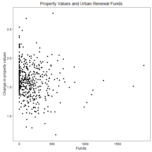
incomePlot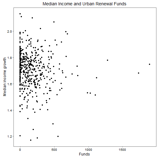
povertyPlot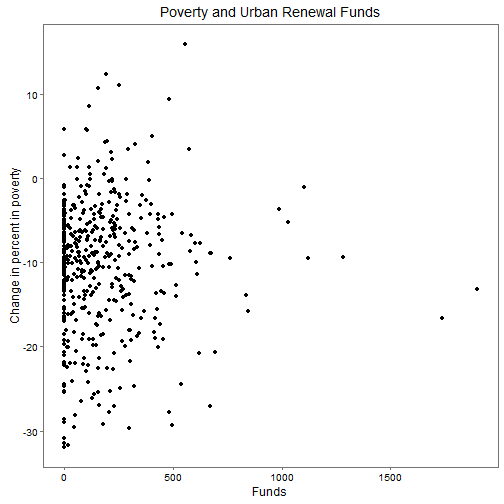
There’s little relationship to see. Clearly if there are relationships, we’ve got to make adjustments to find them. That’s why we’ll use our model to adjust for confounding variables and our instrument.
The Model
To use an instrument variable you use a two-stage regreesion. First model the instrument (years of participation - CODE) against the treatment (urban renewal grants per capita - CODE) to see if the instrument is significant.
Williams and Shester use two models, one simple and one using a lot of economic variables as controls. R comes with the lm function for fitting linear models.
IV.basic <- lm(app_funds_pc50 ~ yrsexposure_UR + Iregion_12 + Iregion_21 + Iregion_22 + Iregion_31 + Iregion_32 + Iregion_33 + Iregion_41 + Iregion_42 , data = city)

IV.advanced <- lm(app_funds_pc50 ~ yrsexposure_UR + pownocc50 + lnmedval50 + pdilap50 + poldunits50 + punitswoplumb50 + pcrowd50 + lnpop50 + pnonwht50 + plf_manuf_50 + pemp50 + medsch50 + lnfaminc50 + pinc_under2g_50 + Iregion_12 + Iregion_21 + Iregion_22 + Iregion_31 + Iregion_32 + Iregion_33 + Iregion_41 + Iregion_42 , data = city)

summary(IV.basic)
##
## Call:
## lm(formula = app_funds_pc50 ~ yrsexposure_UR + Iregion_12 + Iregion_21 +
## Iregion_22 + Iregion_31 + Iregion_32 + Iregion_33 + Iregion_41 +
## Iregion_42, data = city)
##
## Residuals:
## Min 1Q Median 3Q Max
## -280.84 -122.67 -49.75 63.43 1634.29
##
## Coefficients:
## Estimate Std. Error t value Pr(>|t|)
## (Intercept) 0.1506 82.2691 0.002 0.998540
## yrsexposure_UR 9.7062 3.1643 3.067 0.002290 **
## Iregion_12 38.0311 37.9887 1.001 0.317311
## Iregion_21 -136.0565 34.9360 -3.894 0.000113 ***
## Iregion_22 29.0926 46.2369 0.629 0.529534
## Iregion_31 -4.9827 43.5944 -0.114 0.909055
## Iregion_32 -57.1677 51.3320 -1.114 0.266011
## Iregion_33 -30.6077 52.0524 -0.588 0.556817
## Iregion_41 -5.7090 64.2579 -0.089 0.929245
## Iregion_42 -100.8740 42.3983 -2.379 0.017768 *
## ---
## Signif. codes: 0 '***' 0.001 '**' 0.01 '*' 0.05 '.' 0.1 ' ' 1
##
## Residual standard error: 211.8 on 448 degrees of freedom
## Multiple R-squared: 0.1028, Adjusted R-squared: 0.08479
## F-statistic: 5.704 on 9 and 448 DF, p-value: 1.675e-07summary(IV.advanced)##
## Call:
## lm(formula = app_funds_pc50 ~ yrsexposure_UR + pownocc50 + lnmedval50 +
## pdilap50 + poldunits50 + punitswoplumb50 + pcrowd50 + lnpop50 +
## pnonwht50 + plf_manuf_50 + pemp50 + medsch50 + lnfaminc50 +
## pinc_under2g_50 + Iregion_12 + Iregion_21 + Iregion_22 +
## Iregion_31 + Iregion_32 + Iregion_33 + Iregion_41 + Iregion_42,
## data = city)
##
## Residuals:
## Min 1Q Median 3Q Max
## -277.18 -114.38 -52.70 64.16 1572.85
##
## Coefficients:
## Estimate Std. Error t value Pr(>|t|)
## (Intercept) 1920.74917 2009.10063 0.956 0.33959
## yrsexposure_UR 10.32003 3.29919 3.128 0.00188 **
## pownocc50 -2.23714 1.39348 -1.605 0.10912
## lnmedval50 -66.93736 72.07994 -0.929 0.35358
## pdilap50 1.04677 4.32450 0.242 0.80885
## poldunits50 -0.15491 0.84606 -0.183 0.85481
## punitswoplumb50 -0.48007 1.70615 -0.281 0.77856
## pcrowd50 -0.06288 2.64394 -0.024 0.98104
## lnpop50 -3.72301 12.66762 -0.294 0.76897
## pnonwht50 1.54227 1.66560 0.926 0.35498
## plf_manuf_50 -1.14134 1.31213 -0.870 0.38487
## pemp50 -11.02434 7.54419 -1.461 0.14465
## medsch50 4.29208 16.22318 0.265 0.79147
## lnfaminc50 -13.66471 250.95341 -0.054 0.95660
## pinc_under2g_50 -1.16487 5.24609 -0.222 0.82438
## Iregion_12 40.11278 43.22257 0.928 0.35390
## Iregion_21 -94.00924 45.17485 -2.081 0.03802 *
## Iregion_22 57.87116 61.51792 0.941 0.34737
## Iregion_31 -59.19804 66.66550 -0.888 0.37504
## Iregion_32 -123.52933 78.12609 -1.581 0.11457
## Iregion_33 -57.85992 79.06764 -0.732 0.46470
## Iregion_41 -22.98570 77.12064 -0.298 0.76581
## Iregion_42 -123.18947 59.22877 -2.080 0.03812 *
## ---
## Signif. codes: 0 '***' 0.001 '**' 0.01 '*' 0.05 '.' 0.1 ' ' 1
##
## Residual standard error: 211.1 on 435 degrees of freedom
## Multiple R-squared: 0.135, Adjusted R-squared: 0.09123
## F-statistic: 3.085 on 22 and 435 DF, p-value: 4.709e-06In the basic model, we’re testing to see if years of exposure has any affect on the amount of funds spent. We ‘control’ for different census regions to make sure that different areas don’t confuse the effect.
We find yrsexposure_UR has a positive and significant coefficient of 9.7, suggesting that it does make a difference. Considering units, this suggests an additional year of potential projects leads to an addition $9.70 in renewal projects per capita.
In the advanced model, we add more economic controls based on economic factors in 1950. For instance, a city with a high employment rate in 1950 (pemp50) may have used fewer federal funds. We see that employment does have a strong negative effect. So areas with strong employment tend to use fewer federal dollars on renewal projects. This is the sort of effect that we’re trying to remove from our final analysis.
Now we need to use that regression (including controls) and get predicted values of urban renewal grants. We feed those predicted values into another regression to test the effects of the urban renewal grants on different economic outcomes. We test the effects on four different economic variables…
#Get predicted values from the IV model we just created and add them to the data

city$ur_iv <- predict(IV.advanced)

#test outcomes on property values, income, employment, and poverty rates
propertyModel <- lm (lnmedval80 ~ ur_iv + poldunits50 + pdilap50 + punitswoplumb50 + pcrowd50 + pownocc50 + lnmedval50 + pnonwht50 + medsch50 + lnpop50 + lnfaminc50 + pemp50 + plf_manuf_50 + pinc_under2g_50 + Iregion_12 + Iregion_21 + Iregion_22 + Iregion_31 + Iregion_32 + Iregion_33 + Iregion_41 + Iregion_42 , data=city)

incomeModel<- lm (lnfaminc80 ~ ur_iv + poldunits50 + pdilap50 + punitswoplumb50 + pcrowd50 + pownocc50 + lnmedval50 + pnonwht50 + medsch50 + lnpop50 + lnfaminc50 + pemp50 + plf_manuf_50 + pinc_under2g_50 + Iregion_12 + Iregion_21 + Iregion_22 + Iregion_31 + Iregion_32 + Iregion_33 + Iregion_41 + Iregion_42 , data=city)

employmentModel<- lm (pemp80 ~ ur_iv + poldunits50 + pdilap50 + punitswoplumb50 + pcrowd50 + pownocc50 + lnmedval50 + pnonwht50 + medsch50 + lnpop50 + lnfaminc50 + pemp50 + plf_manuf_50 + pinc_under2g_50 + Iregion_12 + Iregion_21 + Iregion_22 + Iregion_31 + Iregion_32 + Iregion_33 + Iregion_41 + Iregion_42 , data=city)

povertyModel<- lm (pinc_under5g_80 ~ ur_iv + poldunits50 + pdilap50 + punitswoplumb50 + pcrowd50 + pownocc50 + lnmedval50 + pnonwht50 + medsch50 + lnpop50 + lnfaminc50 + pemp50 + plf_manuf_50 + pinc_under2g_50 + Iregion_12 + Iregion_21 + Iregion_22 + Iregion_31 + Iregion_32 + Iregion_33 + Iregion_41 + Iregion_42 , data=city)

summary(propertyModel)
##
## Call:
## lm(formula = lnmedval80 ~ ur_iv + poldunits50 + pdilap50 + punitswoplumb50 +
## pcrowd50 + pownocc50 + lnmedval50 + pnonwht50 + medsch50 +
## lnpop50 + lnfaminc50 + pemp50 + plf_manuf_50 + pinc_under2g_50 +
## Iregion_12 + Iregion_21 + Iregion_22 + Iregion_31 + Iregion_32 +
## Iregion_33 + Iregion_41 + Iregion_42, data = city)
##
## Residuals:
## Min 1Q Median 3Q Max
## -0.70599 -0.13073 0.00591 0.12744 0.65489
##
## Coefficients:
## Estimate Std. Error t value Pr(>|t|)
## (Intercept) 1.3814350 2.1203578 0.652 0.51506
## ur_iv 0.0006924 0.0002971 2.331 0.02022 *
## poldunits50 -0.0013056 0.0007849 -1.663 0.09697 .
## pdilap50 0.0012416 0.0040802 0.304 0.76104
## punitswoplumb50 0.0021313 0.0015967 1.335 0.18266
## pcrowd50 0.0012078 0.0024575 0.491 0.62332
## pownocc50 0.0009795 0.0014893 0.658 0.51107
## lnmedval50 0.8906912 0.0715942 12.441 < 2e-16 ***
## pnonwht50 -0.0037329 0.0015725 -2.374 0.01804 *
## medsch50 -0.0114937 0.0152053 -0.756 0.45012
## lnpop50 -0.0510325 0.0117454 -4.345 1.74e-05 ***
## lnfaminc50 -0.0020301 0.2564311 -0.008 0.99369
## pemp50 0.0193466 0.0076807 2.519 0.01213 *
## plf_manuf_50 -0.0032816 0.0012581 -2.608 0.00941 **
## pinc_under2g_50 0.0024053 0.0052561 0.458 0.64745
## Iregion_12 -0.2367832 0.0423415 -5.592 3.97e-08 ***
## Iregion_21 -0.1020339 0.0498359 -2.047 0.04122 *
## Iregion_22 -0.0984661 0.0565752 -1.740 0.08249 .
## Iregion_31 -0.0640967 0.0665157 -0.964 0.33577
## Iregion_32 0.0346612 0.0801918 0.432 0.66579
## Iregion_33 -0.0591041 0.0801599 -0.737 0.46132
## Iregion_41 0.1088341 0.0743790 1.463 0.14413
## Iregion_42 0.4924837 0.0664283 7.414 6.49e-13 ***
## ---
## Signif. codes: 0 '***' 0.001 '**' 0.01 '*' 0.05 '.' 0.1 ' ' 1
##
## Residual standard error: 0.1961 on 434 degrees of freedom
## (1 observation deleted due to missingness)
## Multiple R-squared: 0.7227, Adjusted R-squared: 0.7087
## F-statistic: 51.42 on 22 and 434 DF, p-value: < 2.2e-16summary(incomeModel)##
## Call:
## lm(formula = lnfaminc80 ~ ur_iv + poldunits50 + pdilap50 + punitswoplumb50 +
## pcrowd50 + pownocc50 + lnmedval50 + pnonwht50 + medsch50 +
## lnpop50 + lnfaminc50 + pemp50 + plf_manuf_50 + pinc_under2g_50 +
## Iregion_12 + Iregion_21 + Iregion_22 + Iregion_31 + Iregion_32 +
## Iregion_33 + Iregion_41 + Iregion_42, data = city)
##
## Residuals:
## Min 1Q Median 3Q Max
## -0.56067 -0.04737 0.00851 0.06389 0.28128
##
## Coefficients:
## Estimate Std. Error t value Pr(>|t|)
## (Intercept) 2.336e+00 1.061e+00 2.201 0.028234 *
## ur_iv 2.409e-04 1.609e-04 1.497 0.135189
## poldunits50 5.364e-04 4.253e-04 1.261 0.207830
## pdilap50 1.717e-03 2.204e-03 0.779 0.436333
## punitswoplumb50 1.782e-03 8.646e-04 2.061 0.039892 *
## pcrowd50 -3.394e-05 1.331e-03 -0.025 0.979671
## pownocc50 4.705e-03 8.037e-04 5.855 9.41e-09 ***
## lnmedval50 2.091e-01 3.857e-02 5.422 9.81e-08 ***
## pnonwht50 5.506e-04 8.509e-04 0.647 0.517929
## medsch50 7.631e-04 8.197e-03 0.093 0.925868
## lnpop50 -2.393e-02 6.338e-03 -3.775 0.000182 ***
## lnfaminc50 5.519e-01 1.263e-01 4.371 1.55e-05 ***
## pemp50 1.152e-02 4.161e-03 2.768 0.005883 **
## plf_manuf_50 -1.267e-03 6.812e-04 -1.860 0.063505 .
## pinc_under2g_50 -2.803e-04 2.659e-03 -0.105 0.916102
## Iregion_12 -1.091e-01 2.288e-02 -4.767 2.55e-06 ***
## Iregion_21 -5.578e-02 2.699e-02 -2.067 0.039304 *
## Iregion_22 -3.847e-02 3.065e-02 -1.255 0.210143
## Iregion_31 -4.711e-02 3.600e-02 -1.309 0.191337
## Iregion_32 3.547e-02 4.344e-02 0.817 0.414655
## Iregion_33 -5.016e-03 4.340e-02 -0.116 0.908039
## Iregion_41 -5.847e-02 4.030e-02 -1.451 0.147545
## Iregion_42 -1.459e-02 3.599e-02 -0.405 0.685460
## ---
## Signif. codes: 0 '***' 0.001 '**' 0.01 '*' 0.05 '.' 0.1 ' ' 1
##
## Residual standard error: 0.1063 on 435 degrees of freedom
## Multiple R-squared: 0.6345, Adjusted R-squared: 0.616
## F-statistic: 34.32 on 22 and 435 DF, p-value: < 2.2e-16summary(employmentModel)##
## Call:
## lm(formula = pemp80 ~ ur_iv + poldunits50 + pdilap50 + punitswoplumb50 +
## pcrowd50 + pownocc50 + lnmedval50 + pnonwht50 + medsch50 +
## lnpop50 + lnfaminc50 + pemp50 + plf_manuf_50 + pinc_under2g_50 +
## Iregion_12 + Iregion_21 + Iregion_22 + Iregion_31 + Iregion_32 +
## Iregion_33 + Iregion_41 + Iregion_42, data = city)
##
## Residuals:
## Min 1Q Median 3Q Max
## -14.429 -1.081 0.256 1.223 4.636
##
## Coefficients:
## Estimate Std. Error t value Pr(>|t|)
## (Intercept) 13.265134 20.718757 0.640 0.522349
## ur_iv 0.003367 0.003142 1.072 0.284482
## poldunits50 -0.003343 0.008302 -0.403 0.687354
## pdilap50 -0.050901 0.043027 -1.183 0.237461
## punitswoplumb50 0.044338 0.016879 2.627 0.008922 **
## pcrowd50 0.010319 0.025990 0.397 0.691532
## pownocc50 0.026022 0.015688 1.659 0.097903 .
## lnmedval50 3.702343 0.752941 4.917 1.25e-06 ***
## pnonwht50 -0.049582 0.016611 -2.985 0.002997 **
## medsch50 0.079020 0.160006 0.494 0.621657
## lnpop50 -0.279475 0.123715 -2.259 0.024376 *
## lnfaminc50 1.236503 2.464841 0.502 0.616163
## pemp50 0.403055 0.081235 4.962 1.00e-06 ***
## plf_manuf_50 -0.044481 0.013298 -3.345 0.000895 ***
## pinc_under2g_50 0.038665 0.051905 0.745 0.456728
## Iregion_12 -2.673809 0.446694 -5.986 4.51e-09 ***
## Iregion_21 -3.695338 0.526778 -7.015 8.85e-12 ***
## Iregion_22 -1.796852 0.598403 -3.003 0.002830 **
## Iregion_31 -0.238684 0.702713 -0.340 0.734276
## Iregion_32 -0.372282 0.847945 -0.439 0.660850
## Iregion_33 0.415264 0.847260 0.490 0.624292
## Iregion_41 -2.030569 0.786688 -2.581 0.010173 *
## Iregion_42 -1.178270 0.702629 -1.677 0.094272 .
## ---
## Signif. codes: 0 '***' 0.001 '**' 0.01 '*' 0.05 '.' 0.1 ' ' 1
##
## Residual standard error: 2.074 on 435 degrees of freedom
## Multiple R-squared: 0.5211, Adjusted R-squared: 0.4969
## F-statistic: 21.51 on 22 and 435 DF, p-value: < 2.2e-16summary(povertyModel)##
## Call:
## lm(formula = pinc_under5g_80 ~ ur_iv + poldunits50 + pdilap50 +
## punitswoplumb50 + pcrowd50 + pownocc50 + lnmedval50 + pnonwht50 +
## medsch50 + lnpop50 + lnfaminc50 + pemp50 + plf_manuf_50 +
## pinc_under2g_50 + Iregion_12 + Iregion_21 + Iregion_22 +
## Iregion_31 + Iregion_32 + Iregion_33 + Iregion_41 + Iregion_42,
## data = city)
##
## Residuals:
## Min 1Q Median 3Q Max
## -9.413 -1.776 -0.284 1.453 93.255
##
## Coefficients:
## Estimate Std. Error t value Pr(>|t|)
## (Intercept) 55.145466 72.905664 0.756 0.44994
## ur_iv -0.005810 0.009660 -0.601 0.54793
## poldunits50 -0.074282 0.027161 -2.735 0.00657 **
## pdilap50 0.029969 0.137529 0.218 0.82763
## punitswoplumb50 -0.088867 0.056126 -1.583 0.11428
## pcrowd50 -0.002281 0.081797 -0.028 0.97777
## pownocc50 -0.169103 0.052785 -3.204 0.00149 **
## lnmedval50 -4.316539 2.393598 -1.803 0.07223 .
## pnonwht50 0.110390 0.052143 2.117 0.03499 *
## medsch50 -1.610934 0.533537 -3.019 0.00273 **
## lnpop50 0.356454 0.393696 0.905 0.36590
## lnfaminc50 2.263099 8.636517 0.262 0.79345
## pemp50 0.020153 0.261717 0.077 0.93867
## plf_manuf_50 -0.033093 0.042230 -0.784 0.43381
## pinc_under2g_50 0.045346 0.180496 0.251 0.80179
## Iregion_12 2.930786 1.500507 1.953 0.05163 .
## Iregion_21 -0.009868 1.694326 -0.006 0.99536
## Iregion_22 0.031132 1.971659 0.016 0.98741
## Iregion_31 -2.986668 2.185537 -1.367 0.17268
## Iregion_32 -3.865594 2.615349 -1.478 0.14033
## Iregion_33 -3.918800 2.667494 -1.469 0.14274
## Iregion_41 -0.373342 2.441029 -0.153 0.87853
## Iregion_42 -1.543513 2.183218 -0.707 0.48006
## ---
## Signif. codes: 0 '***' 0.001 '**' 0.01 '*' 0.05 '.' 0.1 ' ' 1
##
## Residual standard error: 5.835 on 336 degrees of freedom
## (99 observations deleted due to missingness)
## Multiple R-squared: 0.2431, Adjusted R-squared: 0.1935
## F-statistic: 4.904 on 22 and 336 DF, p-value: 2.874e-11We can see that the federal programs do have a significant effect on future property values. To interpret this coefficent, you would say that an addition $100 in per capita funding relates to a 6.9% increase in median property values by 1980. Interestingly, the authors get different slightly different standard errors – likely due to OLS calculation specifics – that show the effect on income to be significant while our regression does not. But it relates at $100 increase in spending to a 2.4% increase in median income.
The other economic variables do not show specific effects.
Conclusions
This analysis can not determine whether urban renewal projects are good or bad in all measures. However, it does provide evidence that urban renewal projects boost property values and increase median incomes – for the city as a whole – over an extended period of time.
It remains to be seen whether these economic effects are felt across all income levels and what peripheral costs are imposed up groups with lower incomes.